
A Complete Guide to Optical Transceiver Nomenclature
Decoding the alphabet soup of form factors, reach classifications, modulation schemes, and everything in between.

Welcome to a 🔒 subscriber-only deep-dive edition 🔒 of my weekly newsletter. Each week, I help investors, professionals and students stay up-to-date on complex topics, and navigate the semiconductor industry.
If you’re new, start here. See here for all the benefits of upgrading your subscription tier!
As a paid subscriber, you will also have access to a video explanation of this post, an executive summary with key highlights, perhaps some nano banana illustrations 🍌 and a google drive link to this article so that you can parse it with your favorite LLM.
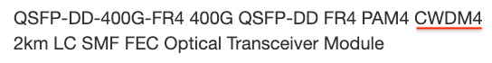
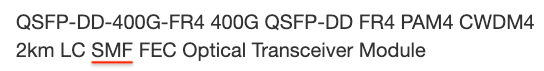
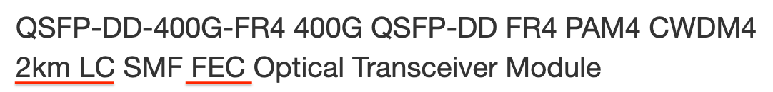
When entering the world of optical transceivers, one quickly runs into an intimidating selection of alphanumeric soups that are confusing to the uninitiated. For example, take a look at this optical transceiver product page from FiberMall.

In this post, we will go through what each of these terms mean in a step-by-step fashion. At the end of this article, you’ll be reading optical transceiver product pages like a seasoned industry professional.
The naming standards you see in this product page originates from the IEEE Ethernet Working Group that defines the electrical and optical specifications at the PHY layer via the IEEE 802.3 standard. The 802.3 is not a single standard, but a whole family with various amendments along the way. At the PHY level, their main purpose is to define the electrical and optical characteristics used in signal transmission - things like optical power, link budgets, acceptable bit error rates, and signal encoding. For instance, the upcoming 802.3dj scheduled for release in spring 2026 defines 200 Gbps, 400 Gbps, 800 Gbps and 1.6 Tbps aggregate bandwidths using 200 Gbps lanes, and is also popularly known as Ultra Ethernet.
The way an optical interconnect is defined most often follows the format below (give or take, because there is no rigid way this is defined in the industry):
[Connector-Form-factor]-[Baseband-Speed]-[Reach][Number of Lanes]-[Modulation]-[Multiplexing]-[FiberMode]-[Other Info]
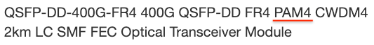
Let’s break down the product name in the example above: QSFP-DD-400G-FR4 PAM4 CWDM4 2km LC SMF FEC, according to the template shown above and dive into every aspect of it.
1) Small Form-Factor Pluggable (SFP)

The first part of the product name corresponds to the form factor of the pluggable connector that houses the optical transceiver. In the example above, QSFP stands for Quad Small Form-Factor Pluggable connector and it looks like the picture below.

The “quad” comes from the fact that it has four independent communication lanes in it. A QSFP+ connector is a faster version of QSFP. The DD in the optical transceiver example above stands for Double Density which means that it can run eight lanes in a quad form-factor effectively doubling the aggregate bandwidth. QSFP-DD connectors are quite widely used in 400G networking.

In 800G networking, the “octal” SFP or OSFP pluggable modules are more common which support eight independent communication lanes. As we transition to even higher speeds like 1.6T or 3.2T, the longer variant called OSFP-XD (extra dense) is more commonly used. In the future, as we make the transition to co-packaged optics (CPO), the size of the pluggable will dramatically drop because most of the transceiver functionality will be co-packaged with the network ASIC switch.

The table below is a handy reference to quickly identify the SFP pluggables most commonly used in optics.

2) Aggregate Data Rates

The “400G” part tells you the total data rate: 400 Gbps. This is the aggregate throughput you get from the entire link that includes four or eight parallel lanes at once. In many cases, you will see this specified as “400GBASE” and the “BASE” here means baseband transmission. It essentially means the signal is transmitted directly without being modulated onto a carrier frequency. It is often dropped for brevity. The aggregate data rate is ultimately what determines how fast the optical interconnect is.
Interconnect speeds have been continuously getting faster, but with the advent of hyperscalars for AI applications, there is a pressing need for even faster interconnects to keep up with compute scaling.

3) Reach Distance

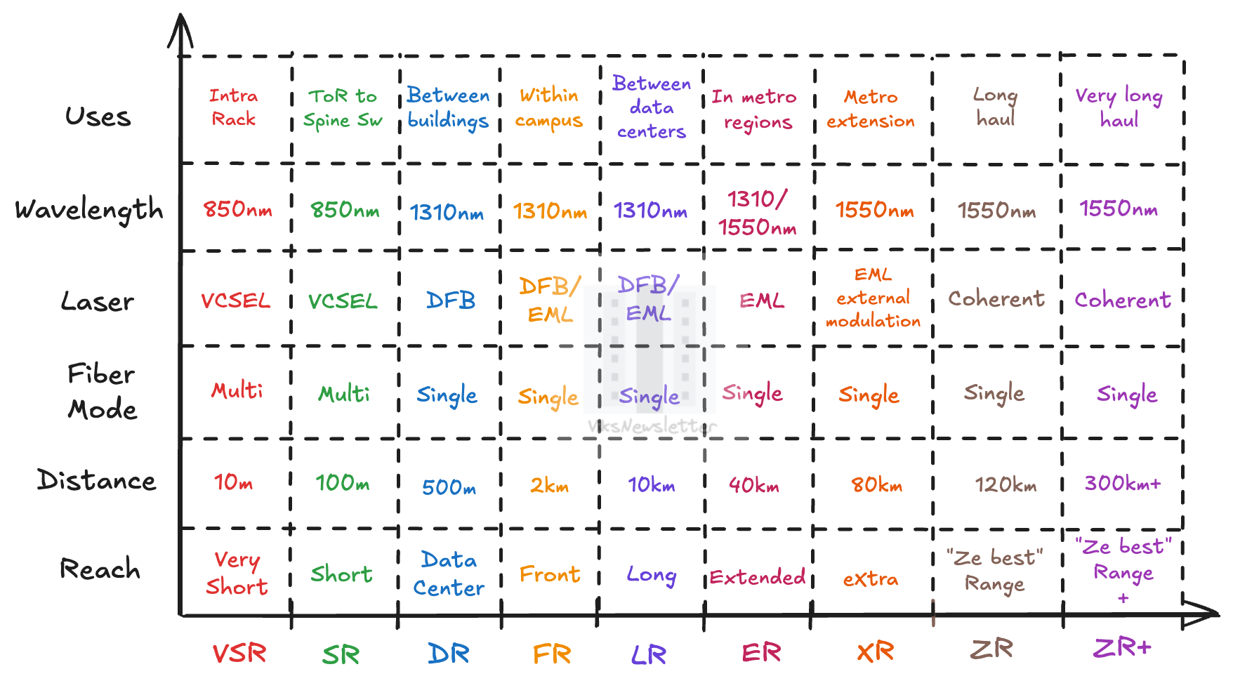
Depending on the optical communication distance, technologies are classified into nine different distance tiers – from very short reach (VSR) commonly used within a single rack in datacenters, to what is playfully called “ze best range” (ZR) interconnects that work over hundreds of kilometers. The boundaries that separate various distance tiers are blurred, and depend a lot on the data rates, modulation schemes, and even the quality of fiber in use. Still, the classifications are generally useful in thinking about different optical technologies.
After the paywall:
A handy chart that shows reach distances, fiber modes, laser types, wavelengths, and use-cases for all nine distance tiers from VSR to ZR+.
Decoding number of parallel lanes and how they translate to aggregate bandwidth.
Multiplexing schemes used to increase aggregate data rates.
Modulation schemes and different kinds of electro-optical modulators.
Different kinds of fiber modes used, and which is used at what distance.
Miscellaneous connector information and specifications.
The picture below shows the use-cases, wavelengths, laser technologies, and fiber type used for every optical distance tier, in a single easy-to-use chart.
In the original example, FR refers to front reach (or fiber/far/fixed reach, they are all used) which means that the optical transceiver will work up to the kilometer range, and is most useful for networking between buildings.
The complexity of optical engineering continuously increases with higher distance tiers. Different wavelengths are used based on the propagation loss as the optical signals travel long distances. Laser sources and detection methodologies get more complex and expensive at higher distances. We will discuss why certain laser sources are suitable to certain lengths in a different article.
4) Number of Parallel Lanes
Earlier we discussed aggregate data speeds only because data is almost always sent via more than one parallel optical link. Sending high data rates over a single lane is often not practical because the engineering gets very complex and circuits involved get power hungry due to the need for error correction. The more the number of parallel lanes in the optical highway, the higher the aggregate bandwidth.
In our optical transceiver example, FR means that the front reach interconnect uses four parallel optical connections to deliver an aggregate bandwidth of 400 Gbps. This means that each optical lane is running at 1/4th the aggregate speed, or at 100 Gbps. Thus, whenever we talk about speeds in optical interconnects it is important to clarify if the numbers refer to “per-lane” or “aggregate” speeds.
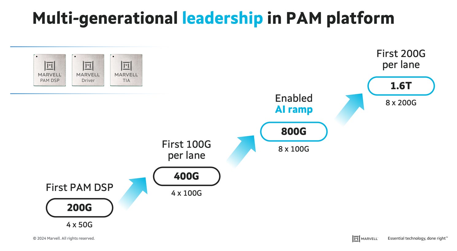
The roadmap from Marvell shown below shows that both per-lane speeds and more parallel lanes are required to increase the aggregate bandwidth in optical links.
6) Multiplexing Schemes
The method used to combine the data from independent parallel lanes into one aggregate connection is called the multiplexing scheme. In our original example, this is indicated by CWDM4 which is the abbreviation for 4-wavelength Coarse Wavelength Division multiplexing. This means that data is transmitted on four different wavelengths simultaneously (often around 1310 nm wavelengths - specifically: 1271/1291/1311/1331nm) on a single optical fiber.
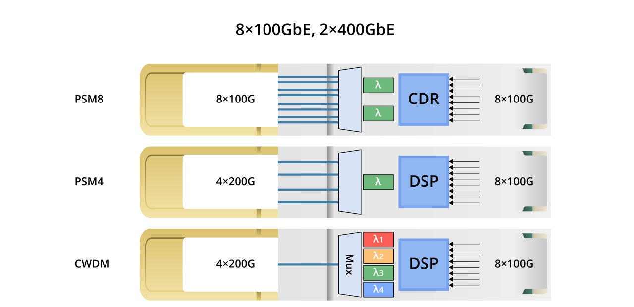
A more straightforward way to achieve parallel connections is to simply add more physical optical fibers all operating at the same wavelength. This is called Parallel Single Mode (PSM) and the figure below shows the implementation of multiplexed parallel lanes with both multiple fibers, single wavelength and single fiber, multiple wavelength. The obvious downside of PSM is that there is a lot of fiber to manage and complex connector assemblies that can fail. The middle ground is running each fiber at a higher data rate, which means fewer fibers are needed for the same aggregate bandwidth.
For extremely long reach (ZR, ZR+) interconnects, the implementation of parallel lanes gets much more complex. They often use Dense Wavelength Division Multiplexing (DWDM) which implements 100+ wavelengths around 1550nm (C-band) over a single optical fiber, and are amplified by Erbium-Doped Fiber Amplifiers (EDFAs) for long-haul optical networks. These often require large equipment boxes to perform such dense multiplexing.
A big source of excitement in the optical industry is the recent introduction of 400G-ZR standard which introduces DWDM for datacenter interconnects in a compact pluggable connector running at 400G aggregate speeds. This will be a separate post in the future.
5) Modulation Schemes
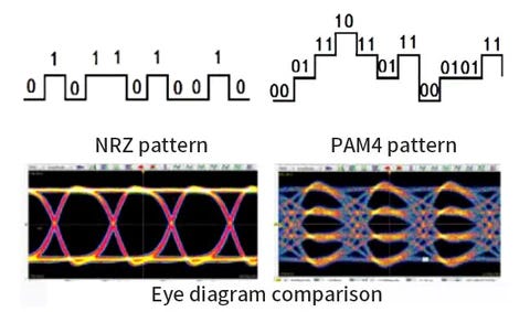
Modulation refers to the method used to convert electrical 0s and 1s to light. The simplest method is to use On-Off Keying (OOK): turn off the laser to represent a 0, and turn it on to represent a 1. The signal is then transmitted as a set of pulses that is decoded by the receiver. This simple approach is effective when the data rates are low - in the range of 50 Gbps.
At data rates of 100 Gbps and beyond, the fiber distorts the optical signal and it becomes difficult to turn on and off lasers so quickly. This also depends on the speed and intended reach of the optical interconnect: faster and longer interconnects require complex modulation formats, and expensive DSP techniques that are power hungry.
In such scenarios, a different modulation scheme like 4-level Pulse Amplitude Modulation (PAM4, like in our optical transceiver example) is used. Here two bits are taken at a time - like 00, 01, 10, or 11 - and are encoded as four different laser brightness levels.
There are two fundamental ways to generate a modulated signal in an optical transceiver: direct laser modulation, and external modulation.
Direct Laser Modulation
Different levels of laser output can be obtained by adjusting the laser drive current to four different levels. Higher drive currents above a certain laser threshold current generate more photons, and a brighter laser output. Most often, the lowest level in PAM4 modulation does not involve turning off the laser by setting drive current below laser threshold because turning on a laser has dynamic effects that result in signal distortions. Instead, the lowest level is often a “dim” laser output that is still above the threshold. The figure below shows different levels of optical output power based on the drive (or injection) current from a laser diode.
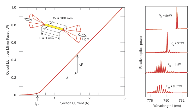
This power-current dynamic of laser sources is usually very sensitive to temperature, and thus the amount of drive current always needs to be monitored in a feedback sensing loop to ensure that the output power for a given modulation level is consistent.
External Modulation
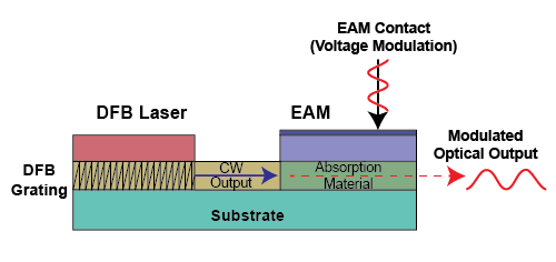
The other way to modulate signals is to keep the laser output power constant, and use an external modulator to control the level of light entering the fiber. This approach often gives better waveforms compared to direct laser modulation, but is also more complex and expensive when a separate modulation device is needed. External modulators are a fascinating topic which we won’t get into great depth here. Suffice to say that there are three basic types of modulators with entirely different operating principles:
Electro-absorption modulators: Depending on the applied electric field, these modulators absorb different levels of light. Different laser intensities can be coupled into the fiber by controlling the level of absorption via an electrical signal thereby creating a PAM4 signal.
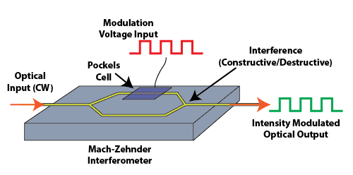
Mach-Zehnder Modulators (MZMs): These modulators split light into two parallel paths and use the principle of interference to couple different levels of light into fiber. Destructive interference causes a dim level of laser output to be coupled in the fiber while constructive interference produces bright light.
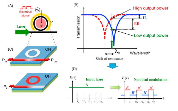
Ring Modulators: These modulators are extremely compact compared to MZMs and are a great fit for silicon photonics. The basic idea is to put a ring close to the main path of the laser signal. Depending on the refractive index it is built on and when sized properly, the ring can completely “trap” the signal from the main path via resonance providing low laser output. A voltage applied to the material can change the refractive index, and change the resonant frequency of the ring. This means that the main wavelength is no longer “trapped” by the ring, and thus produces a bright output. The same principle can be applied to generate intermediate brightness levels for PAM4.
It is good to understand the different modulation methods that are used in optical transceivers, but the actual method used is not often mentioned in the name. There is a lot behind the design and performance of these modulators that is beyond the scope of this post.
7) Fiber Modes
There are broadly two kinds of fiber used in datacenters and anywhere optical networks are needed: Single Mode Fiber (SMF) and Multi Mode Fiber (MMF).
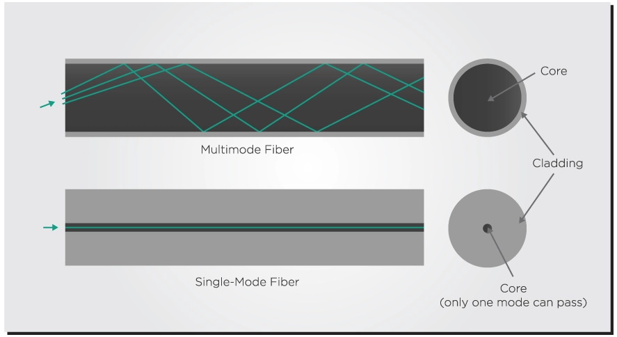
When laser sources such as vertical cavity surface emitting lasers (VCSELs) are used, they emit a wide cone of laser light that is often coupled into a MMF. MMFs are usually pretty thick optical fibers that are 10s of micrometers in diameter. Each ray of light in the wide laser cone can take a different path through the optical fiber. Some rays go directly through, while others bounce around the fiber quite a bit and arrive late.
This means that a pulse sent into a MMF “spreads” as it travels to the other end because each “mode” of light arrives at a slightly different time, which implies that you can’t send closely spaced pulses in a MMF fiber because they would spread and merge into each other. The farther the optical interconnect, the more these pulses spread. This phenomenon introduces two limitations:
If pulses cant be sent close to each other, then interconnect speed becomes limited.
They are only useful for short reach interconnects where spreading isn’t significant.
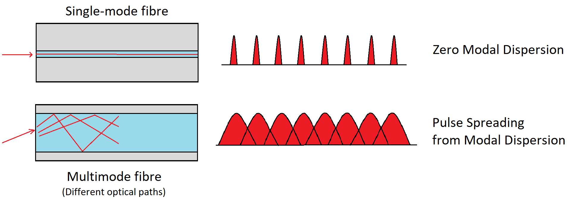
There is a variant of the MMF called graded-index MMF where the refractive index of the glass core continuously decreases with distance from the center. These are called OM3/OM4 fibers, and they minimize pulse spreading by allowing light along longer paths to travel at higher speeds so that all the modes of the pulse arrive at the same time, or nearly so.
A SMF fiber on the other hand is much thinner - often under 10 micrometers in diameter. This limits the light propagation to a single mode (they can still have different polarizations - a subtlety to note) which means that the spreading will be minimal. SMF is better for faster optical interconnects, and for distances above 100m. They are also significantly more expensive, and much more difficult to align lasers with narrow diameter SMF.
8) Miscellaneous
Optical transceivers often have a mish-mash of other information that depends on the manufacturer or vendor. Things like:
Reach distance, like 2 km that is mentioned in our example, which is already implicit in the “FR” classification
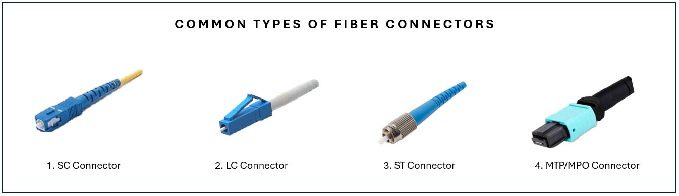
The kind of optical fiber connector that connects into the SFP connector is also often mentioned - in our example, this is the Lucent Connector, or LC. Depending on the application, there are other types of connectors that are commonly used as shown in the picture below.
As the reach distance of the interconnect increases, DSP functions are often required to recover the signal correctly. Techniques like Forward Error Correction (FEC), amplification, clock-data recovery (CDR) and equalization are employed to compensate for signal distortions, and correctly extract the right symbol sequence with a low bit error rate (BER).
This covers most of what is needed to understand the product definitions and specifications of optical transceivers used for datacenter, telecom and long haul applications. I’m sure I missed something because this nomenclature is a bit of the wild-west. Let me know in the comments if I can clarify something.
Hope this was helpful! 🍻
so which stocks are best to buy now eventhough they are up big