
A Primer on Transformer Architecture: Model Parameter Calculations, Estimating GPT-5 Architecture
A detailed look at transformers, the role of attention, and decoder-only architecture; Learning to count model parameters based on architecture and making guesses on GPT-5 internal construction.

Welcome to a 🔒 subscriber-only deep-dive edition 🔒 of my weekly newsletter. Each week, I help investors, professionals and students stay up-to-date on complex topics, and navigate the semiconductor industry.
If you’re new, start here. As a paid subscriber, you will get additional in-depth content. We also have student discounts and lower pricing for purchasing power parity (see discounts). See here for all the benefits of upgrading your subscription tier!
P.S.: I usually post these on Sundays, but since the post was ready and GPT-5 was released, I decided to ship it! Enjoy.
GPT-5 is here: with the sloppy plots, the major buildup, and subsequent disappointment. It’s not the quantum leap it was made out to be, but is another waypoint in the evolution of AI models. But every successive generation seems to grow in size.
GPT-2 had about a hundred million parameters in 2019. In just about four years, the parameter count crossed one trillion with GPT-4. GPT-5, whose model architecture is undisclosed, is expected to be in the range of 5-10 trillion parameters — give or take. There are no public numbers to back up these claims.
Without a formal background in AI/ML, there is a vague sense that larger is better. So far, this has held true. But, a curious engineering mind poses other questions: What are these parameters? How are they chosen? How come they’ve gotten so big?
In this post, we will answer these questions with a foundational understanding of Transformer architecture used in LLMs, their inner workings, and conclude with a back-of-the-envelope model parameter counting approach that will be able to account for 99% of the parameters used in GPT models, without the rigor of a more formal approach. We’ll use the learning to take a stab at the architecture of GPT-5. YMMV.
This post is aimed at readers without a background in machine learning concepts. The emphasis is on acquiring a basic understanding of LLMs and model parameters, and learning to make rough calculations to appreciate what goes on inside an LLM.
For free subscribers:
Birth of the Transformer: A short introduction describing how it all started in 2017 that frames the discussion to follow with historical context.
Tokens, Embeddings and Vocabulary: How sentences are broken up, converted to numbers, and form a table of all words that an LLM understands.
QKV, Context Window, and Batch Sizes: Understanding the key components required to calculate Attention, what context window means, and why batches are important for training.
Attention Calculation Methods: We will look at scaled dot-product attention, and how that is modified to calculate multi-headed attention — a common approach in transformer-based LLMs.
Decoder Transformer Architecture: Understanding the internals of the commonly used “decoder-only” architecture in LLMs like ChatGPT.
For paid subscribers:
Parameter counting using Google’s BERT-Base. We will go through step-by-step and count all the 110 million parameters in the weight matrices used in this early LLM. We will provide a generic formula that is applicable to most model architectures like ChatGPT.
Detailed look at GPT2/GPT3: Using published model architecture for early OpenAI models, we will calculate and verify the number of parameters used in GPT2 and GPT3 models.
An educated guess at GPT4: While OpenAI did not openly publish model weights for GPT4, several industry experts have guess its model architecture. We will use these estimates to make detailed parameter calculations on GPT4.
Speculating on GPT5: We don’t know anything about internal model architecture, but we can look at the evolution of GPT models to make educated guesses and estimate the total parameter count.
References: A list resources I found useful to learn transformer architecture from the basics.
Downloadable Google Sheet you can use to make your own parameter estimates and speculate on GPT-5!
Read time: 18-20 mins
Birth of the Transformer
The concept of a Transformer was introduced in a revolutionary paper by Google in 2017 called Attention is all you need, which is considered the starting gun for the modern AI race.
The problem addressed in the original paper is language translation from English to German, which is a notoriously hard problem due to the way grammar and sentences work. Serialized word-for-word translation does not produce meaningful results, nor is it efficient. For any given word in a sentence, the context of what comes before and after is important. To emulate this awareness, Google researchers introduced the concept of Attention in the context of a neural network (a mathematical imitation of how our brains work) which they referred to as Transformer (only because it sounded cool.)
The authors soon realized that the Transformer is capable of much more than translation. It could generate meaningful conversation and generate insights when asked to do so. They also recognized that this approach also applies to audio, images and video, and that the larger this Transformer is made, the better it works. The surprising power of a large language model almost feels like an accident.
It scaled beautifully to larger architectures because Attention requires multiplying arrays of numbers called matrices — which, as it turns out, we are really good at doing with computer chips. Today, we are looking at using hundreds of thousands of CPUs and GPUs to make chips think and do our jobs for us.
But the process begins with converting human language to the world of numbers, so that we can use chips to perform calculations that allow silicon to think at extraordinary scale. We’ll look at how this works next.
Tokens, Embeddings, and Vocabulary
Since computers work well with numbers, a sentence is first broken up and encoded into in floating point numbers — which is computer-speak for a number with several decimal places. A sentence could be separated according to words, syllables, punctuations or spaces, and each piece is called a token. Similar representations are possible for images, text or video.
Once the input is broken up into tokens, it must be converted to an array of numbers called a vector using the process of embedding. How big this array of numbers or vector is (a quantity labeled dk), depends on the choice of transformer architecture.
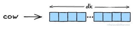
For example, Deepseek R1 full model uses an embedding size of 7,168 floating point numbers. Smaller variants of this model could use lower sizes. GPT-4 likely uses close to 16,000 numbers. The choice of size is critical: too small and it fails to capture intricate relationships between words; too large, and memory requirements explode.
The collection of all possible embeddings (think of it as the number form of words) represents the total dictionary of words that the LLM understands, and is referred to as the vocabulary of the model. Deepseek R1 has a total vocabulary size of 129,280 tokens. The total embedding table size is product of token embedding size and vocabulary length. Here it is 7,168 × 129,280 floating point numbers. This large array of numbers is essentially the “Oxford Dictionary of English” that an LLM will use.
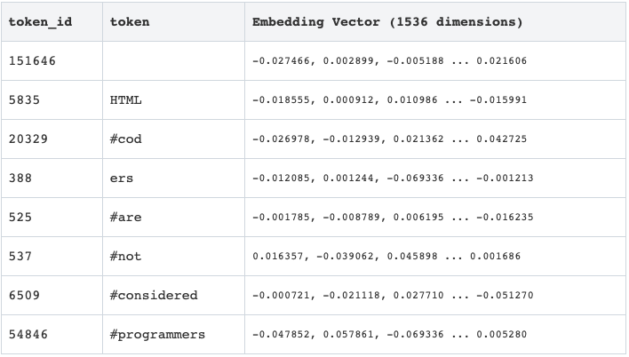
The table below shows the token embeddings for the sentence “HTML coders are not considered programmers.”
Each floating point number in an embedding can be represented at different levels of precision:
Higher precision like float32 (FP32) uses 4 bytes.
Half precision formats like float16 (FP16) uses 2 bytes.
Low precision formats like int8 uses 1 byte.
Higher precision is excellent for training the model, but comes at high memory cost. Lower precision is good for memory savings, and useful for fast inference (a term for using the trained model to generate outputs.) The choice of precision is important to ensure that the LLM will run on the available hardware.
QKV, Context Window, and Batch Sizes
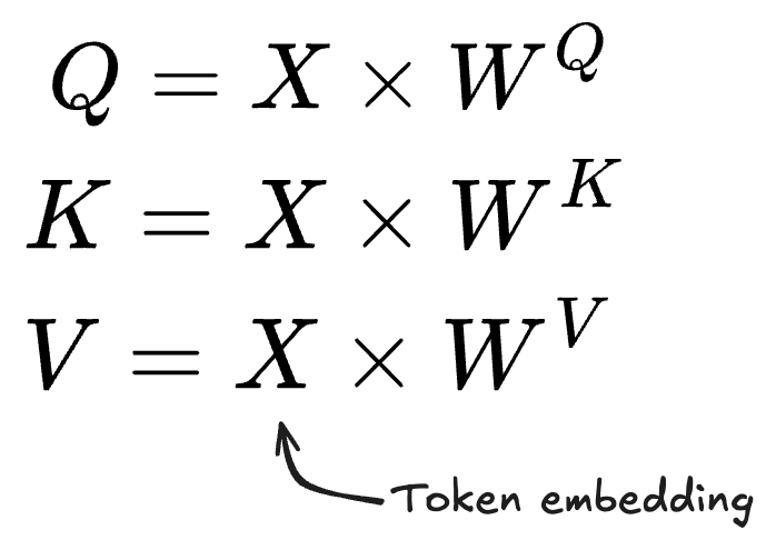
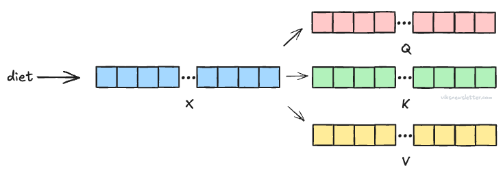
Once a token has been embedded into numeric vector format, three unique quantities called Query, Key and Value are then calculated for each embedding, say X. These new vectors (Q, K, V) are essential for computing Attention, and are obtained from the matrix multiplication below.
Broadly speaking, we can assign meaning to these quantities as below:
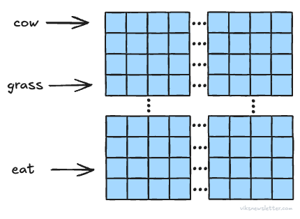
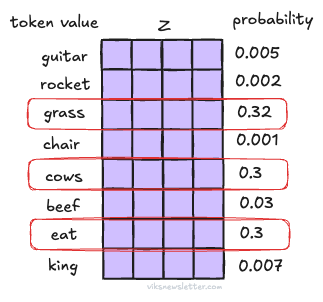
Query (Q): This vector is the equivalent of asking - “Which of the tokens in the sequence are relevant to my input token X (say diet)?”
Key (K): This vector is the response to the query identifying the indices of the tokens that are relevant — “Tokens 124, 908, and 1,423 are relevant.”
Value (V): This vector provides the content of each of those tokens — “Token 124 says cow, Token 908 says grass, Token 1,423 says eat.”
The picture above shows the Q, K, V vectors for one token X. In practice, many tokens are taken together and processed at once. We will discuss exactly how.
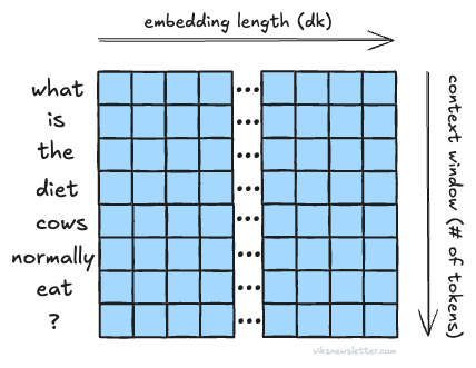
Every row in the matrix X corresponds to a single token embedding like a word. The number of rows depends on how many tokens are taken together — a metric called sequence length or context window. For example, Google’s Gemini 2.5 Pro uses 1 million tokens in its context window during inference, which corresponds to 1 million row entries in the matrix X. Assuming an embedding vector length of 3,092 and 1 million rows, X is a 2D matrix of size 3,092 × 1 million.
Context window helps the model remember what was presented to it 1 million tokens ago, which means it can draw meaning between a lot of tokens. This is critical when you give an LLM a whole book and ask for a summary, or require it to remember long conversations. Such long context windows are good for inference, but not for training.
To speed up the process of training, models process multiple sequences simultaneously in batch sizes anywhere between tens to hundreds. Context windows used for model training will be considerably shorter — like 8,000 to 32,000 tokens — to keep the memory requirements during training in check.
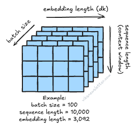
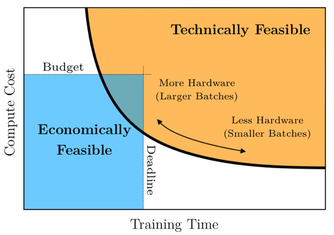
As an example: assuming a batch size of 100, sequence length of 10,000 tokens, and token vector length of 3,092, X becomes a 3D matrix of size 3,092 × 10,000 × 100, or about 3 billion floating point numbers. Using larger batch sizes speeds up the training process, which smaller batches are computationally more feasible. This Pareto frontier explains the trade-off nicely.
The matrices WQ, WK and WV are called weight matrices and are obtained from the training process using a method of back-propagation which we won’t get into here. Their sizes are based on the embedding vector length, dk.
For example, with a 4,096 element long vector like the one used in the GPT3-6.7B model, the weight matrices are of size [4,096 × 4,096]. The means that the Q, K, V matrices calculated from the matrix multiplication equation shown above will also be 4,096 elements long per token, which will expand along three dimensions when context window and batch size is taken into account.
Scaled Dot-Product Attention
With Q, K, V matrices available, the important quantity called Attention as proposed by Google researchers can be calculated using the following function.
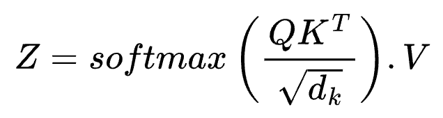
Let’s understand this equation better by looking at its components.
Query × Key (Transposed): This is the dot product of the query and key matrices, which requires taking a transpose of the matrix for the math to work. The resulting vector has many numbers, each of which gives you a measure for how well what you asked (query) aligns with what is in the tokens (key). A high value at any point in the vector means there is a lot of relevance; a low value means there is little relevance.
√dk: dk is the length of the token embedding which could be 4,096 like in GPT3-6.7B. The dot product is divided by the square root of this embedding to scale the dot product values down to smaller numbers.
softmax: This is a mathematical function that converts any vector of length L into a probability of L possible outcomes. After applying the softmax function, the values in the scaled dot-product have probability values between 0 and 1.
Dot-product with V: By computing the dot product of the probabilities of token relevance with the token value vector, you get the probabilities of how relevant each token in the context window is to the original query.
We have now computed Attention, and based on how we took the dot product and scaled it, this method is called scaled dot-product attention. From our earlier example, words like cow, grass, and eat will have a high relevance to diet, but a word like chair will not. This also underlines the important of large context windows in making intelligence connections between words; a large context window will find more relevance to tokens and draw meaning from them.
Multi-Headed Attention
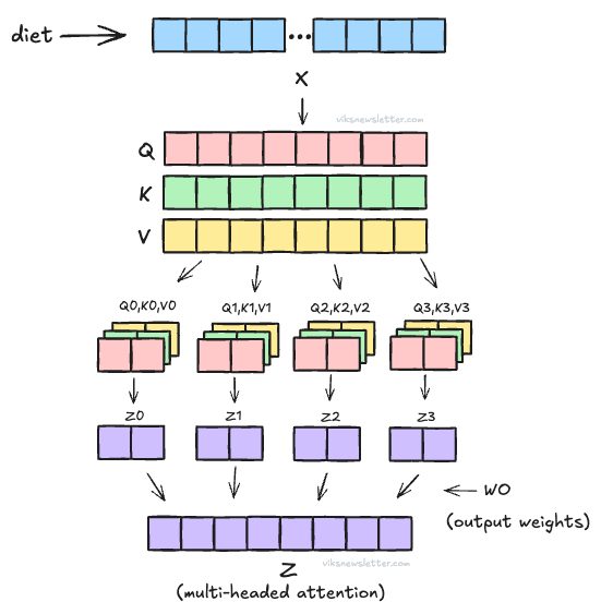
A better way to capture complex relationships between tokens and improve performance of LLMs is to use multi-headed attention. This is the attention calculation approach adopted by most LLMs today. The step-by-step process looks like this:
Compute Q, K, V matrices from the input embedding X like before.
Logically break up these matrices into multiple smaller matrices called heads, and calculate attention on each head.
Reconstruct the large attention matrix by joining together attention from each head.
For example, Q, K, V matrices of size 2,048 can be broken up into 16 heads. This means that size of vectors in each head is 2,048/16 = 128 floating point numbers. The same process of scaled dot product attention described earlier is applied to each of the 16 heads. The attention from each head is then collected at the output to form multi-headed attention. More specifically, it is multiplied by another weight matrix WO before getting the final attention Z. The picture below shows this process for four heads.
Decoder Transformer Architecture
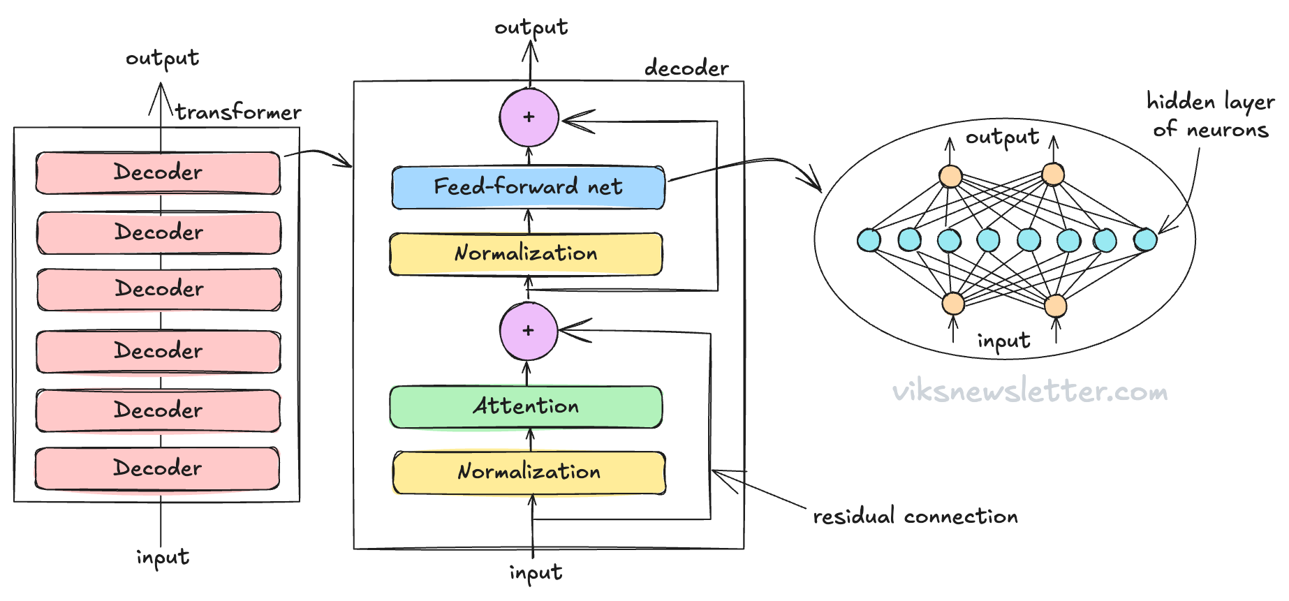
With what we’ve learned so far, we can now discuss the decoder-only architecture, which is used by OpenAI models such as ChatGPT-4. The decoder is a fundamental building block of a transformer, and has three components.
Attention (which we have already discussed)
Feedforward network (FFN)
Normalizations and residual connections
A multi-layer Transformer is built by stacking several decoders. The input to the first decoder is word embeddings — the translation of tokens into numbers, but every subsequent decoder gets the output of the previous decoder as input. The figure below shows a transformer with 6 layers of decoders.
Feedforward Network
The feedforward network or FFN (sometimes called the multi-level perceptron or MLP) is a two-layer neural network. It is called feedforward because information only moves from input to output, and never backwards.
If you’re not familiar with the idea of a neural network, it is the mathematical representation of the complex structure of a biological brain.
There are neurons represented by little circles in the complex mesh of connections inside the FFN. Each connection is the equivalent of a synapse between any two neurons, represented by a mathematical function called the activation function. The activation function has several constant parameters associated with it, and these are called weights of the FFN which are usually obtained from the LLM training process.
The illustration shows orange circles as the input/output neurons and the blue circles as hidden-layer neurons. This network is called a two-layer FFN because there are two layers of weights — one from input to hidden layer, and another from hidden layer to output. The choice of the number of neurons in the hidden layer of the FFN is an important architectural choice in the design of Transformer-based LLMs.
Normalization and Residual Connections
These steps are present to maintain a stable numerical environment during the calculation process. As numbers pass through the decoder, they may explode into large numbers unless constrained by the process of repeated normalization at each step. This is a key requirement to getting transformers to work, without which it becomes extremely difficult to scale to larger networks. Residual connections involves adding the input to the output so that the gradients (how fast numbers change) are kept under control in the training process. We’ll leave it at that level of detail for now.
After the paywall, we will use these concepts to calculate the number of parameters in popular LLMs. Specifically, we will cover:
Parameter counting using Google’s BERT-Base. We will go through step-by-step and count all the 110 million parameters in the weight matrices used in this early LLM. We will provide a generic formula that is applicable to most model architectures like ChatGPT.
Detailed look at GPT2/GPT3: Using published model architecture for early OpenAI models, we will calculate and verify the number of parameters used in GPT2 and GPT3 models.
An educated guess at GPT4: While OpenAI did not openly publish model weights for GPT4, several industry experts have guess its model architecture. We will use these estimates to make detailed calculations on GPT4.
Speculating on GPT5: There is plenty of online hype about GPT5 and how it is going to be game-changing. We will take a conservative look at the probable model architecture for GPT5 and estimate the total parameter count.
References: A list of useful references to learn transformer architecture from the basics.
Paid subscribers also get a downloadable Google Sheet you can use to make your own parameter estimates and speculate on GPT-5!